Help
4. Theoretical Background
4.1 Introduction to the Physics of Plasma4.2 Principles of the Plasma Chemistry
4.3 Monte Carlo method in simulation of electron kinetics
4.4 Description of used cross-sections
4.5 The electron-electron interactions
4.1 Introduction to the Physics of Plasma
A gas under normal conditions always contains several hundred charged particles, generated for example by cosmic rays. A gas containing ions and free electrons is called 'ionized gas'. Under special circumstances, it can turn to be plasma. Plasma is also a collection of neutral and charged particles, but it must satisfy criteria presented in this subsection.To produce plasma it is necessary to liberate electrons that are normally bound into atoms. There are various means whereby the energy necessary for ionization may be added to the bound electron. Ordinarily the energy comes from collision events. Two predominant processes are electron, or photon collisions.
Produced charged particles posses Coulomb fields through which they interact with each other and with electric and magnetic fields externally applied. This interaction causes them to react in a collective manner to forces. This collective behavior constitutes the prime characteristic of plasma.
Electric field of individual charged particle is effectively shielded by the oppositely charged particles in its neighborhood. The distance where the field of single charged particle is already shielded is called Debye distance, D:
where k is the Boltzman constant, T is the effective temperature of particles of charge e in Kelvin (K), of which there are n per unit volume. Thus, one quantitative criterion for the existence of plasma is that the linear dimension of the system, L, has to be large enough compared to D:
And this shielding can be effective only if the number of charged particles within a sphere of radius D is much greater than one:
Quasi-neutrality is another criterion for the existence of plasma:
where ni are the number of positive ions and ne number of electrons per unit volume.
Basic characteristics of plasma are the density of charged (n) and neutral (ng) particles, the temperatures of the neutral and charged particles Tg, Te and T+ respectively.
According to the density of charged particles one speaks about weakly ionized plasma, if ng >> n, or about strongly ionized plasma (ng < n).
According to the temperature, plasmas are divided to high temperature plasmas with T > 106 K (stars and thermo-nuclear fusion) and low temperature plasmas with T < 106 (gas discharges, ionosphere...).
A term non-thermal plasma is used for the plasmas where Te >> Tg and T+ respectively. The plasma where these temperatures are approximately equilibrated is called thermal plasma.
Among these various plasma types, the non-thermal plasma has been applied to induce chemical reactions in various otherwise inert gaseous mixtures (for example flue gas treatment, the generation of ozone ...), because of its non-equilibrium properties, low power requirement and its capacity to induce physical and chemical reactions within gases at relatively low temperatures.
The laboratory plasma used for these purposes is usually generated by the ionization or breakdown of a neutral gas by application of various electric and magnetic fields. Under the action of applied electric field ions and the electrons present in the gas move in opposite directions through it.
By doing so, they suffer collisions with other ions, electrons and neutral particles. The ions, because of their greater mass, do not gain much velocity from the applied field and the energy they posses is easily transferred to the neutral atoms by elastic collisions.
Electrons, on the other hand, acquire and maintain their velocities easily and if the voltage drop across the discharge tube is sufficiently great, electrons can gain sufficient energy between two collisions to produce additional ionization and excitation.
The electrons in a non-thermal plasma can reach temperatures of 10,000 - 100,000 K (1 - 10 eV), while the gas temperature can remain as low as room temperature. It is the high electron temperature that determines the unusual chemistry of non-thermal plasmas.
4.2 Principles of the Plasma Chemistry
Fast (or hot) electrons are key factor in plasma chemistry. These electrons collide with molecules of background gas and some of these collisions leads to the formation of radicals, ions or excitated states. In next step, these reactive intermedaite species can initiate another reactions, which can lead to the formation of final stable products.
So, first of all, we need to know more about possible processes resulting from electron impact on neutral molecules (or atoms) of background gas. These processes include (there are more electron involving reactions, including interaction with ions, other electrons and surfaces, but it is not the scope of this help to discuss this problem):
e + A → A* + e (excitation - rotational, vibrational, electronic)
e + A → A+ + e + e (ionization)
e + A → A- (electron attachment)
e + AB → A + B + e (neutral dissociation)
e + AB → A+ + e + B + e (dissociative ionization)
e + AB → A- + B (dissociative attachment)
These processes are characterized by their cross-sections and threshold energies. And because the energy of chemical bonds is in order of several eV, the mean electron energy must at least 2 - 3 eV, in case we want to use plasma to initiate chemical reactions in otherwise inert gaseous mixtures.
And as I have already written, electron can get this energy from externally applied electric fields. In homogenous fields, if work in done on an electron, it gains energy
where vd is a drift velocity. And the energy eV can be gained by moving distance d in the electric field E:
However, this distance d is a random number. The average distance between two collisions is called mean free path (λ). In the first approximation, if we consider only elastic collisions and atoms (or molecules) are represented as hard spheres with radius r, the mean free path is given by formula:
where ng is the concentration of neugral particles and σ represents a cross-section of each atom (σ = π.r2).
In reality, this cross-sections is not a constant, but it depends on the energy (velocity) of impacting electron. And as I have already written, each type of collision (elastic, excitation, ionization...) is characterized by its own cross-section.
So, the calculation of mean free path, and also mean energy of electrons is more complicated and it requires a knowledge of a distribution function of electron velocities. On the other hand, because electron loses different amounts of energy as a result of different types of collisions, this velocity distribution function of electrons depends strongly on the cross-sections of individual processes.
Velocity distribution function is defined in such a way, that the number of electrons in the generalized volume d3rd3v close to {r,v} is given by:
From this distribution function, any other quantity can be calculated later. Electron energy distribution function (EEDF) may also be derived from it. EEDF, f(r,ε) is defined in such a way, that the local fraction of electrons in the energy range (ε, ε + dε) is given by
The EEDF is very important for the chemical kinetics in plasmas. For an elementary binary reaction between electrons and atoms A, the rate of the reaction (i. e. the number of elementary reactions taking place per unit time and unit volume) is given by
where nA is the number density of A, ne is the electron number density and k is the rate coefficient, given in turn by
where f is the EEDF, me is the electron mass and σ is the cross-section of the elementary process, εth is the treshold energy.
In cold plasmas, these distribution functions can have strongly non-Maxwellian shape. But they satisfy well-known Boltzmann equation. So, one way how to get this distribution functions is to numerically solve this equation. The second approach is to use so called Monte Carlo concept for this purpose.
4.3 Monte Carlo method in simulation of electron kinetics.
Monte Carlo methods are widely used for complex physical and mathematical problems. Examples of Monte Carlo approaches in the field of gas discharges have been given by several authors. The trajectory of electrons in a reactor configuration can be computed by means of a Monte Carlo algorithm [Bra92], [Has91], [Pal91], [Sat91].The so called zero-collision Monte Carlo method, originally developed by Skullerud [Sku68], is frequently used to compute plasma parameters, see [Him92], [Wen90], [You92].
The similarity of results obtained by Monte Carlo methods and the numerical solution of the Boltzmann equation was shown by Segur et al [Seg84]. They stressed the necessity of using more than the first four terms of the spherical harmonic expansion in the solution of the Boltzmann equation.
I have also decided to use Monte Carlo simulation instead of solving Bolzmann equation. I have based my script on the algorithm presented by Marnix A. Tas [Tas95]. So, I am first going to describe his algorithm and then I will describe changes I have made there.
The basis of the Monte Carlo algorithm used in their paper is a re-definition of the EEDF. Usually, the EEDF is defined as the energy distribution of an assembly of N electrons at time t1. They state that, under identical conditions, the same EEDF is found when the energy of a single electron is sampled at N moments in time. In one respect this approach is better than the conventional one because here the initial energy has to be chosen for one electron only. Its value, however, does not have a great influence since it is lost within a few collisions. The electron then continues on its way with a realistic energy value.
In their program MCED, the gas mixture in which the electron motion is simulated is modeled as a uniform matrix of gas molecules. Each molecule is positioned in a cubic unit cell with volume Vm = 1/n, so the distance of molecules is δs = Vm1/3.
The electron motion under the influence of the electric field from one molecule to another is straightforward. Random numbers
determine the type of these molecules and whether interaction between electron and these molecules occurs or not.
Random numbers also determine type of eventual collision.
These random numbers are derived from cross-sections of induvidual elementary processes. For example, the collision probability
of the test electron with the energy ε with a molecule m is given as a ratio of the sum of cross-sections
of all possible types of collisions and the area of a side of unit cell:
They have approximated the amount of energy electron gets from electric field as it travels distance δs according to the following schema:
δp|| = δs.E/(2p*) if ε ≥ E.δs
δp⊥ = 0
where p* = √ε denotes the momentum in the unit cell used in their program MCED, δp|| and δp⊥ are the changes of momentum of the electron respectively parallel and perpendicular to the electric field E.
What concerns my script, I had to written it from scratch, because I do not have a source code of program presented by Tas and his co-workers. I also test the probability of interaction of test electron with a molecule of background gas after it passes distance δs. The biggest difference is that the movement of this electron in my script is not straightforward. I re-calculate new direction of his movement after each cycle of calculation (one cycle means change of electron position by distance δs) and in case of collision with a molecule, I use another random number to to determine his new direction.
So, I do not need to use their approximative schema to determine the change of energy of the test electron during one cycle of calculation. I calculate it from basic principles (dv = adt).
The overall algorithm can be summarized in following schema:
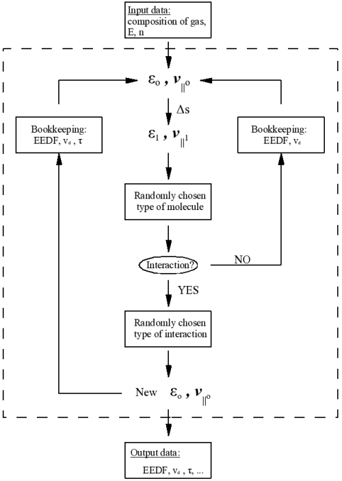
So, as the out come we have EEDF, drift velocity (vd) and mean time between collisions (τ). Additionally, a reduced mobility of electrons (µ) is derived from drift velocity:
where nl is Loschmidt´s constant. From the τ, it is also possible to calculate frequency of collisions (ν = 1/τ). What concerns electron mean energy, it is already calculated from the final EEDF, not during the simulation, despite the fact, that I also store the information about the mean electron energy calculated during the simulation as an average from energies the test electron had during each cycle of the simulation. But these energies are slightly different, and now I am going to explain you why.
As I have already mentioned, the approach I am using to calculate EEDF is a re-definition of Monte Carlo method, since I did not focus on energy of a large ensemble of electrons, but on one electron sampled at N moments in time. But because I check its energy after he passes distance E.δs and not after equal time steps E.δt, when this electron has higher energy (and thus also higher velocity), higher energies are sampled more frequently. That is why primary produced EEDF has to be scaled down by the factor of velocity.
MySQL table created during the calculation contains numbers, which tell us, how many times during the simulation has the test
electron energy from given interval. These intervals are not equal. So, to produce final normalized EEDF (stored in *.csv file),
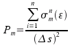
the number
stored in MySQL table has to be devided by the interval widths, scaled down by velocity factor
(√ε) and finaly normalized, so that:
where number of energy intervals is p and the width of interval j is δj. However, script for the analysis can deal with both types of data, so you can use it to calculate additional parameters from counts of electron occurance in each energy interval stored in MySQL table, as well as from final normalized EEDF stored in a *.csv file.
Apropos, the number and widths of these energy intervals is given by files stored in directory '/intervals', and you must choose one of them at the beginning of the calculation. But you can also create your own files with division of energy to intervals. It is very easy, just have a look on the form of one of these files, for example normal.txt, and you will know how to do it.
What concerns additional analysis of produced EEDF, as I have already mentioned in section 2.2 (Additional analysis of calculated EEDF), you can use script 'Analysis' to get drift velocity, frequency of collisions, electron mean energy, mean free path, electron mobility, reduced electron mobility, rate constant of all elementary electron processes included in the simulation and energy branching. They are calculated according to the following formulae:
Mean electron energy:
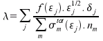
Mean free path:
Frequency of collisions:
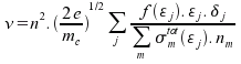
Drift velocity:
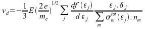
where m represents index of a molecule, σmtot is the sum of all cross-sections for molecule m at given energy and nm is number of molecules m per unit volume. All remainig variables were already mentioned before.
4.4 Description of used cross-sections.
I use a set of electron collision cross sections recommended by Sakai [Sak02] for needs of low temperature plasma modeling. I have gained them from a compilation which is available on the anonymous FTP site ftp://jila.colorado.edu/collision_data/. This data has been developed over many years by A.V. Phelps and his coworkers at JILA (Joint Institute for Laboratory Astrophysics). I have update only cross-sections for CO2 according to data published by Yukikazu Itikawa [Iti02]. And in the future, I would like to update cross-sections for H2O.Now, I am going to list all processes, which I have included in my cross-sections. As the name of these processes, I am going to use names of columns in MySQL tables where cross-sections of these processes are stored.
N2:
| qm | momentum transfer |
| qr | rotational excitation, energy loss 0.020 eV, lower limit 0.0, upper limit 5.005 |
| qv1, qv1b | 1st vibrational excitation qv1 - energy loss 0.290 eV. lower limit 0.258. upper limit 80.006, but in the energy range from 1.6 to 3.999 eV, qv1b - energy loss 0.291 eV |
| qv2 | 2nd vibrational excitation, energy loss 0.59 eV, lower limit 1.677, upper limit 3.612 |
| qv3 | 3rd vibrational excitation, energy loss 0.88 eV, lower limit 1.677, upper limit 3.406 |
| qv4 | 4th vibrational excitation, energy loss 1.17 eV, lower limit 1.883, upper limit 3.302 |
| qv5 | 5th vibrational excitation,energy loss 1.47 eV, lower limit 1.883, upper limit 3.406 |
| qv6 | 6th vibrational excitation, energy loss 1.76 eV, lower limit 2.193, upper limit 3.199 |
| qv7 | 7th vibrational excitation,energy loss 2.06 eV, lower limit 2.296, upper limit 3.509 |
| qv8 | 8th vibrational excitation, energy loss 2.35 eV, lower limit 2.477, upper limit 3.509 |
| qe1 | electronic excitation, N2 A3SIGMA, v=0-4, energy loss 6.17 eV, lower limit 5.986, upper limit 150.001 |
| qe2 | electronic excitation, N2 A3SIGMA, v=5-9, energy loss 7.00 eV, lower limit 6.785, upper limit 150.001 |
| qe3 | electronic excitation, N2 B3PI, energy loss 7.35 eV, lower limit 6.992, upper limit 150.001 |
| qe4 | electronic excitation, N2 W3DELTA, energy loss 7.36 eV, lower limit 7.198, upper limit 150.001 |
| qe5 | electronic excitation, N2 A3SIGMA, v=10+, energy loss 7.8 eV, lower limit 7.585, upper limit 150.001 |
| qe6 | electronic excitation, N2 BPRI3SIGMA, energy loss 8.16 eV, lower limit 7.998, upper limit 150.001 |
| qe7 | electronic excitation, N2 APRI1SIGMA, energy loss 8.40 eV, lower limit 8.179, upper limit 500.004 |
| qe8 | electronic excitation, N2 A1PI, energy loss 8.550 eV, lower limit 8.282, upper limit 999.002 |
| qe9 | electronic excitation, N2 W1DELTA, energy loss 8.89 eV, lower limit 8.488, upper limit 150 |
| qe10 | electronic excitation, N2 C3PI, energy loss 11.03 eV, lower limit 10.784, upper limit 150 |
| qe11 | electronic excitation, N2 E3SIGMA, energy loss 11.88 eV, lower limit 11.481, upper limit 150 |
| qe12 | electronic excitation, N2 ADPRI1SIGMA, energy loss 12.25 eV, lower limit 11.997, upper limit 999 |
| qe13 | electronic excitation, N2 SUM of singlet states, energy loss 13 eV, lower limit 12.487, upper limit 999 |
| qi | ionization, threshold energy 15.6 eV, lower limit 12.487, upper limit 999 |
O2:
| qm | momentum transfer |
| qa | SUM OF TWO AND THREE-BODY ATTACHMENT, LOWER LIMIT = 0.000 , UPPER LIMIT = 100 |
| qr | SINGL LEVEL ROT PKQ FOR 300K ENERGY LOSS = 0.020 , LOWER LIMIT = 0.026 , UPPER LIMIT = 1.677 |
| qv1 | ENERGY LOSS = 0.190 , LOWER LIMIT = 0.181 , UPPER LIMIT = 5.005 |
| qv2 | ENERGY LOSS = 0.380 , LOWER LIMIT = 0.439 , UPPER LIMIT = 5.005 |
| qv3 | ENERGY LOSS = 0.570 , LOWER LIMIT = 0.671 , UPPER LIMIT = 44.995 |
| qv4 | ENERGY LOSS = 0.750 , LOWER LIMIT = 0.748 , UPPER LIMIT = 14.990 |
| qe1 | SING DELTA, ENERGY LOSS = 0.977 , LOWER LIMIT = 0.929 , UPPER LIMIT = 100.001 |
| qe2 | B SINGLET SIGMA, ENERGY LOSS = 1.627 , LOWER LIMIT = 1.496 , UPPER LIMIT = 100.001 |
| qe3 | ENERGY LOSS = 4.500 , LOWER LIMIT = 4.386 , UPPER LIMIT = 14.990 |
| qe4 | ENERGY LOSS = 6.000 , LOWER LIMIT = 5.882 , UPPER LIMIT = 100.001 |
| qe5 | ENERGY LOSS = 8.400 , LOWER LIMIT = 8.282 , UPPER LIMIT = 100.001 |
| qe6 | ENERGY LOSS = 9.970 , LOWER LIMIT = 9.778 , UPPER LIMIT = 100.001 |
| qe7 | 130 nm line, ENERGY LOSS = 14.700 , LOWER LIMIT = 14.500 , UPPER LIMIT = 100.001 |
| qi | ENERGY LOSS = 12.060 , LOWER LIMIT = 11.894 , UPPER LIMIT = 100.001 |
CO2:
| qm | momentum transfer |
| qv1 | vibrational excitation - asymmetric stretch, energy loss 0.083 eV lower limit = 0.05 eV, upper limit = 20.009 eV |
| qv2 | vibrational excitation, energy loss 0.167 eV lower limit = 0.167 eV, upper limit = 20.009 eV |
| qv3 | vibrational excitation, energy loss 0.291 eV lower limit = 0.277 eV, upper limit = 99.994 eV |
| qv4 | vibrational excitation, energy loss 0.339 eV lower limit = 1.386 eV, upper limit = 5.065 eV |
| qv5 | vibrational excitation, energy loss 0.252 eV lower limit = 2.394 eV, upper limit = 5.998 eV |
| qv6 | vib. excit., energy loss 0.422 eV lower limit = 2.394 eV, upper limit = 4.511 eV |
| qv7 | energy loss 0.505 eV lower limit = 2.394 eV, upper limit = 4.511 eV |
| qv8 | energy loss 2.50 eV lower limit = 2.394 eV, upper limit = 4.511 eV |
| qa | dissociative ettachment, lower limit = 3.3 eV, upper limit = 10.0 eV |
| qe1 | electronic excitation, energy loss 7.000 eV lower limit = 6.880 eV, upper limit = 11.012 eV |
| qe2 | electronic excitation, energy loss 10.5 eV lower limit = 10.382 eV, upper limit = 99.994 eV |
| qi | ionization, energy loss 13.3 eV lower limit = 13.18 eV, upper limit = 99.994 eV |
H2O :
| qm | momentum transfer |
| qv1 | vib excitation (bending), energy loss = 0.198 eV, lower limit = 0.178, upper limit = 200 |
| qv2 | vib excitation (stretching), energy loss = 0.469 eV, lower limit = 0.432, upper limit = 100 |
| qe1 | energy loss = 1.100 eV, lower limit = 4.877, upper limit = 6.604 |
| qda | dissociative attachment, energy loss = 5.6 eV, lower limit = 5.486, upper limit = 100 |
| qe2 | energy loss = 6.3 eV, lower limit = 6.198, upper limit = 11.1 |
| qe3 | energy loss = 9 eV, lower limit = 8.89, upper limit = 19.99 |
| qe4 | energy loss = 12 eV, lower limit = 11.887, upper limit = 24.994 |
| qe5 | energy loss = 12.5 eV, lower limit = 12.395, upper limit = 100 |
| qi | ionization, energy loss = 12.6 eV, lower limit = 12.497, upper limit = 100 |
4.5 The electron-electron interaction.
If the degree of ionization is set to be higher than 0, the test electron can also interact with surrounding background electrons, which are considered as an isotropic fluid, with a certain background EEDF. What concern the Monte Carlo algorithm, these background electron are treated as if you add a new type of molecules to the mixture, with just one type of interactions described by so called Coulomb cross-section, σc, taken from Mitchner and Kruger [Mit73]:b = e2/(4π.εo.εcoll), λ = (εo.kT/nee2)1/2
where εo is the permitivity of vacuum, ne the electron density, and e the unit charge. The collisional energy, εcoll, is calculated by the scheme of Hashiguchi [Has91]:
where εt and εb are the energy of the test and background electron respectively. The incitent angle θ is taken randomly assuming an isotropic velocity distribution. The energy exchange between these electrons is aproximated by the scheme of Weng and Kushner [Wen90]. These equations could be reduced to:
δεt = - εt.U[0..1] , if εt ≥ εb
where U[0..1] is a random number between 0 and 1.
Unfortunately, at low energies, the Coulomb cross-section becomes very large and it can easily exceed the dimension of the unit cell δs2. So, in this case the probability of the electron-electron interaction would be higher than 1. Therefore, I have decided, that during the each cycle, it is first randomly decided, whether any of electron-molecule interactions will occur. And only if none of these interactions happens, new random number determines the occurence of electron-electron interaction. As a consequence, electron-electron interaction is always underestimated in Web-EEDF.